Amongst Cyber attackers and penetration testers, obtaining a reverse shell on a remote machine is considered a ‘home-run’. Once the reverse shell has been obtained, the remote machine is at the mercy of the attacker. Existing attack platforms such as Metasploit, Empire, and others offer myriad techniques and implementations for obtaining different types of reverse shells. These platforms are powerful and highly configurable, availing the attacker a variety of ‘off-the-shelf’ tools. This means defenders face the extremely difficult task of defending against this arsenal of reverse shell techniques.
A typical reverse shell is obtained using a malicious payload. The payload finds its way into the attacked machine in a variety of ways. Once the malicious payload has been executed it attempts to connect to its server (pre-configured into the payload). Once connection has been established the attacker with access to the server can execute commands via the reverse shell that has been created. Therefore, a common characteristic of reverse shell attacks is the remote connection which yields some sort of communication. Moreover, each command and response should result in some sort of communication side-effect alongside it.
In this article, I’ll describe a method to detect different implementations of a reverse shell with extremely high accuracy and incredibly low False-Positive rate.
Note: this analysis uses intermediate signal-processing and statistics, I’ll attempt to explain intuitively these tools, however, some outside reading might be necessary.
Understanding the signals:
First, we need to understand the nature of these signals. A remote shell allows a remote attacker to execute CMD commands on the attacked machine. On the communication level we should expect a command to be sent to the remote terminal, yielding a packet(s) with the encoded command to be executed to be sent to the attacked machine. Then the command is executed on the remote machine. Once execution is complete and the output is ready, the terminal sends it back to the attackers’ machine.
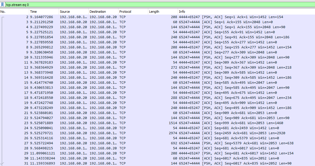
Figure 1: Kali pcap Wireshark view. 192.168.60.100:4444 – kali, 192.168.60.20 – attacked machine. Note both time and size periods as the stream starts.
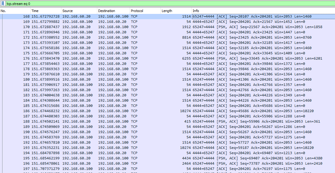
Figure 2: Once the communication reaches a stable point it’s easier to observe the size period. Note that the bigger packets with the wanted information making their way to the Kali machine
Unfortunately, signals don’t follow a specific pattern and can be highly affected by method of transmission, bandwidth, latency and network load. This makes the task of capturing ‘behaviour’ based on observed communication more difficult than simply trying to fit observed packets into specific patterns.
Here’s an example of some non-malicious communication output which ‘behaves’ similarly to remote shell.
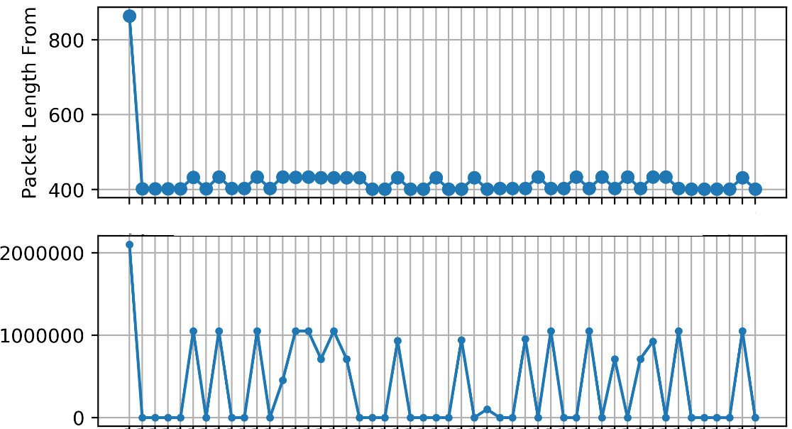
Figure 3: an example of Send-Execute-Return (SER) signal, note the substantial difference of packet size as well as the high correlation between the signals. Note the upper signal is the received packets while the bottom one represents the sent packets
Therefore, if we wish to detect reverse shell we need to use advanced signal processing tools which will not be affected as much as specific ad-hoc pattern look up. In addition, incorporating a Machine-Learning model on top of these signal processing features will allow us to find a fine balance between detection and false positive (detecting a benign communication as malicious). The model will aid us by creating a complex set of rules in order to differentiate each communication.
Enough chatter! Let’s dive into a couple of the main features!
Cross-correlation.
Discretely (which is our case), cross-correlation is defined as:
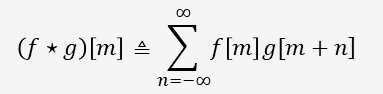
While f, g are signals
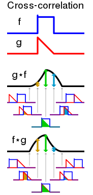
Figure 4: Represents two signals and their cross-correlation. Note that all signals are assumed to be finite (Source: Wikipedia)
When dealing with an SER (Send-Execute-Return) signal (f, g), the normalized (with the max signal length) max value of the cross-correlation is expected to have a high peak at some special ![]()
![]() where represents the delay between the signals. Essentially representing the common processing time of each command. I use this
where represents the delay between the signals. Essentially representing the common processing time of each command. I use this![]() as well as the value
as well as the value ![]() in order to fingerprint the signals. Non-SER signals are expected to have significantly lower max correlation value as a result of the nature of the signals. In addition, non-SER signals are expected to be
in order to fingerprint the signals. Non-SER signals are expected to have significantly lower max correlation value as a result of the nature of the signals. In addition, non-SER signals are expected to be ![]() markedly different than SER signals.
markedly different than SER signals.
(![]() would probably be higher while
would probably be higher while ![]() would be significantly lower)
would be significantly lower)
Fourier Transform
Unequivocally, one of the most important tools of Signal Processing is the Fourier Transform. Fourier transform represents a given time-based signal![]() as a frequency-based signal
as a frequency-based signal![]() . Where
. Where ![]() where
where ![]() operator is described as follows:
operator is described as follows:
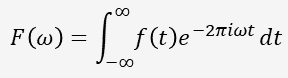
This operator projects ![]() onto the unit circle (by multiplying with
onto the unit circle (by multiplying with ![]() ), integrating over the result yields ‘center of mass’ which maximizes over the ‘base frequencies’ of
), integrating over the result yields ‘center of mass’ which maximizes over the ‘base frequencies’ of ![]() .
.
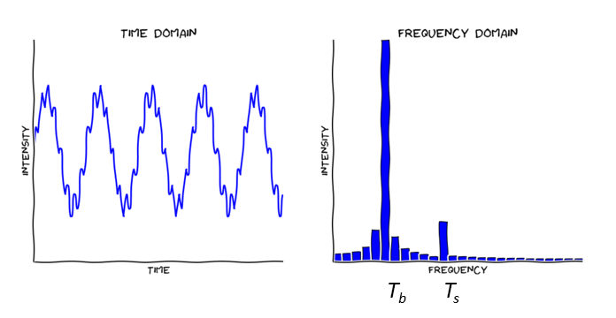
Figure 5: ![]() to the left and
to the left and ![]() to the right as FT example.
to the right as FT example. ![]() has two different periods. The bigger period
has two different periods. The bigger period ![]() yields 5 peaks while
yields 5 peaks while![]() yields many more (while smaller in amplitude).
yields many more (while smaller in amplitude). ![]() peaks at
peaks at ![]() respectively. (Source: adafruit)
respectively. (Source: adafruit)
Similarly, consider the following signal:
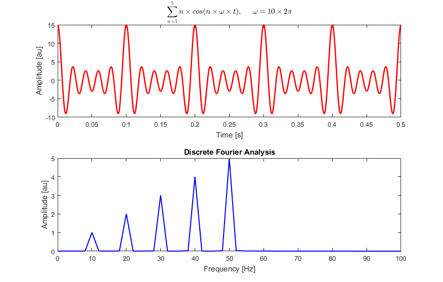
Figure 6: for every period of ![]() ,
, ![]() accumulatively peaks at its’ periodic value. As more period accumulates in the same period the strength of the signal increases. (source: Wikipedia)
accumulatively peaks at its’ periodic value. As more period accumulates in the same period the strength of the signal increases. (source: Wikipedia)
Fourier Transform is a fundamental tool in digital signal processing and allows signal manipulations and analyses which would have been much more difficult in the time domain (![]() ).
).
Following the FT introduction let’s go back and take a look at a (short) malicious signal we’re attempting to analyze:
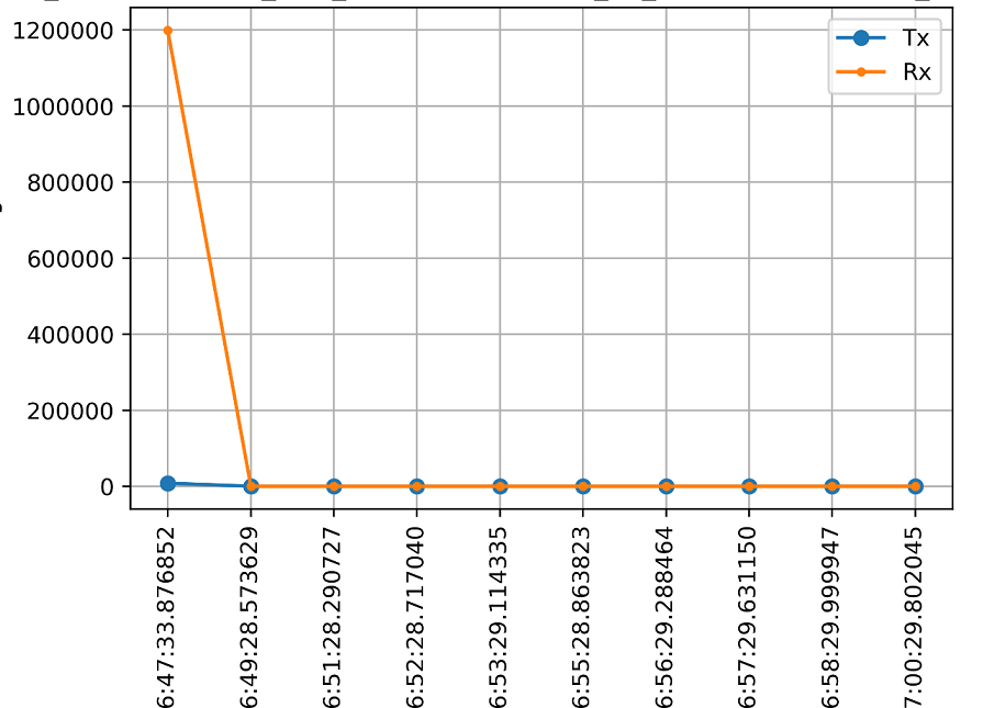
X axis – time[H:M:S:ms], Y axis – packets’ size [bytes]
Figure 7: short idle Metasploit TCP reverse Meterpreter socket sample. Following the handshake, the packets are relatively periodic (a period of 1 minute with skips)
This fundamental behavior is observed (with different parameters) under different implementations of reverse shell Meterpreter as well as Empire’s varied reverse shell implementations. Some implementations allow ‘jitter’ which randomizes packet transmissions time ![]() according to the given parameter. Note that for a small enough jitter (relative to the signal basic period) we would detect the fundamental period even with the usage of jitter, given a long enough sample.
according to the given parameter. Note that for a small enough jitter (relative to the signal basic period) we would detect the fundamental period even with the usage of jitter, given a long enough sample.
I compute the FFT (fast Fourier transform); then take the real part, complex part and absolute value into account when creating a model which describes specific implementation of reverse shell activity.
Note: It is critical to mention that FFT assumes a signal is sampled evenly every ![]() . Because the nature of our data (digital packets) we cannot fulfill this critical prerequisite. Some tweaks were needed in order to ‘aid’ the FFT at its’ task. One attempt to overcome this issue was to manually imitate the FFT process by using histograms to place each packet in a different bucket. Bucketing the packets, as each bucket would represent a different period and the number of packets within each bin would represent the period’s magnitude. The main issue with this method was resolution/performance. In order to allow the ML model to use this feature, it had to be precise in order to achieve better separation when fingerprinting the communication. Theoretically, using smaller and smaller bins would solve the resolution issue but would introduce complexity issue while calculating this feature.
. Because the nature of our data (digital packets) we cannot fulfill this critical prerequisite. Some tweaks were needed in order to ‘aid’ the FFT at its’ task. One attempt to overcome this issue was to manually imitate the FFT process by using histograms to place each packet in a different bucket. Bucketing the packets, as each bucket would represent a different period and the number of packets within each bin would represent the period’s magnitude. The main issue with this method was resolution/performance. In order to allow the ML model to use this feature, it had to be precise in order to achieve better separation when fingerprinting the communication. Theoretically, using smaller and smaller bins would solve the resolution issue but would introduce complexity issue while calculating this feature.
What was used in practice was a 3D Fourier Transform with (packet number, packet size, detection time) as the (x,y,z) axis. This tool allowed us to encapsulate more data into the max ‘period’ as it fuses both size and time into a single parameter. This allowed better separation and feature importance showed that it was one of the top features!
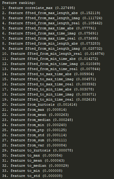
Figure 8: random forest feature importance
Finally, in order to create a robust model, I have collected different basic statistics (standard deviation (SD), mean, max, kurtosis etc.) with the main goal of decreasing the False-Positive rate.
Creating a dataset
To test the effectiveness of the abovementioned task a comprehensive dataset is needed. With the help of the Cyberbit Malware Research Team, we created a small virtual network. One PC in that network was a Kali Linux machine (used for Penetration Testing). We created different kinds of payloads which were stored on an attacked machine (Windows 10). We’ve used Metasploit as well as Empire to generate these payloads. From Kali we recorded the traffic in promiscuous mode while establishing different reverse shells. We tagged the communication based on a known port which we configured while generating the payload.
After establishing a connection, we executed a series of network-awareness, process enumeration, injections and other steps in order to create a varied dataset (different actions were taken each time).
Packet captures (PCAPS) from a large known secured network were collected to create the benign tags. The communication from these different endpoints was tagged as benign.
Only sockets with sufficient information were used.
Machine learning
After building the dataset and extracting different features we need to use them to differentiate between malicious and benign PCAP samples. Roughly ~35 features are computed for each socket (with sufficient samples). These features are then fitted using Random Forest. Random forest is an easy to use machine learning tool since it is relatively straightforward to understand its’ internal mechanism given the data distribution, especially when dealing with a high dimensional dataset.
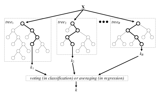
Figure 9: random forest illustration. Each tree predicts whether a given sample is malicious or benign followed by majority voting (Source: ResearchGate)
Results
Given our dataset and Random Forest classifier, the following results were obtained:
Accuracy: 98.99%
The probability of agreements expected by chance: 62.49% of the observations
This yields a very good kappa score of ~1! Like any responsible researcher, I too am naturally suspicious of results that seem too good to be true, so I have suggested some ways that future experiments can be improved in the notes below. I hope this reverse shell detection method will continue to be rigorously tested and improved.
Notes:
- Datasets should be collected from larger, more robust samples and include different types of transmission (WiFi, 4G, etc.). These transmission types are less reliable and may produce substantially different results when observing the signal.
- The model is ‘overfitted’, the model has learned very-well what Metasploit and Empire reverse shells look like. This process should be repeated in order to enable detection of additional reverse shell implementations.
Oriel Zabar is a Machine-Learning researcher at Cyberbit